Introduction
Policy debates often focus only on major decisions made in Washington, DC. But for many Americans, the decisions made much closer to home have just as large, if not larger, effects on day-to-day life. In important respects, the United States remains true to its original system of federalism: states and localities play a prominent role in setting policies that affect the economy more broadly.
State and local government total expenditures amount to $2.9 trillion in the United States. While this is less than the federal government’s $4.3 trillion of expenditures, nearly two-thirds of federal total expenditures are transfers (either to individuals or state and local governments). This means that state and local governments have in some respects a more prominent role in decision-making than the federal government. Indeed, state and local governments make key investment decisions—about infrastructure, education, and many other areas—that help determine the long-run capacity of the entire economy.
State and local governments also enact laws and regulations that define how economic activity takes place. These range from labor market rules to tax policy to environmental regulations to zoning rules. In addition, policymakers’ decisions about how to allocate resources—to education, transportation, or other public goods—are crucial to the U.S. economy. Although the federal government, either by law or by general practice, is required to do extensive analysis of the rules and regulations it makes, this is not always true at the state and local levels. The choices made across states—and sometimes local jurisdictions in the same state—often vary widely.
For housing and transportation policy in particular, decisions made at the local level can have dramatic effects on how and where people choose to live and work. Mobility across states has declined sharply in the United States, and one reason appears to be that land-use restrictions in economically successful regions make it difficult for many workers to move to these locations. Similarly, transportation resources are not always efficiently allocated, making it more difficult for workers to access high-quality jobs.
For the economy to grow and living standards to rise, it is crucial to have successful policy at all levels of government. A set of state and local policy proposals released in January 2019 is the latest in a series of efforts by The Hamilton Project to support broadly shared economic progress through the careful analysis of local, state, and federal policies. This document provides context for those policy proposals in the form of nine economic facts about how state and local policies matter for growth. These facts highlight how rigorous cost-benefit analysis, optimal transportation policy, and land-use rules can affect access to opportunity.
Chapter 1. Economic Significance of State and Local Policies
Fact 1: State and local government budgets are large and represent a sizable portion of the economy.
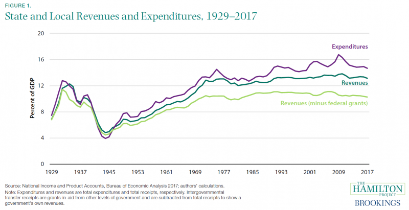
The federal government often receives a disproportionate amount of attention in national discussions of public budgets. In 2017 it collected $3.8 trillion and spent $4.3 trillion, equal to 19.7 percent and 22.3 percent of GDP, respectively (Bureau of Economic Analysis [BEA] 2017; authors’ calculations). By contrast, state and local governments collected and spent amounts equal to 13.1 percent and 14.7 percent of GDP, respectively, representing a significant portion of government total revenues and expenditures. [1]
Figure 1 shows state and local revenues and spending as a fraction of GDP, with federal grants broken out separately. Much of federal spending—about 61 percent in 2017—actually consists of transfers to individuals or to state and local governments (BEA 2017; authors’ calculations). Federal transfers to state and local governments have been increasing since the 1960s, as shown in the gap between revenues and revenues minus federal grants in figure 1. Total receipts at the state and local levels are 28 percent higher when accounting for intergovernmental transfers (BEA 2017; authors’ calculations). [2] Consequently, local and state policies and policymakers are often responsible for the efficient and effective use of public funds. On the other hand, state and local governments may sometimes have limited control over their expenditures, as in the case of Medicaid (which constitutes nearly 30 percent of state expenditures).
Federalism also allows for a wide variety of models for raising and spending revenues. In particular, states and localities employ a diverse assortment of revenue collection methods, including property taxes (primarily at the local level) and individual and sales taxes (at both state and local levels). On average, 16 percent of state and local revenues (not including federal transfers) are derived from personal income taxes and 46 percent are derived from property and sales taxes (including excise taxes).[3] But some states (such as Florida and Alaska) collect no personal income taxes and some states (such as New Hampshire and Oregon) collect no sales taxes (Census 2016b).[4] This results in a relatively low overall state and local tax burden in some states—for instance, 5.7 percent of state GDP in Alaska—and a relatively high burden in other states—as in New York, at 11.5 percent. State and local spending also varies widely, from 15.3 percent of state GDP in Georgia to 32.1 percent in Alaska (Census 2016b; authors’ calculations).
Across states, the share of revenues coming from the local versus the state level also varies widely, from a low of 19 percent coming from the local level in Vermont to a high of 55 percent in Florida (Census 2016b; authors’ calculations). In Florida, which collects no income taxes, localities raise a relatively large amount of money to provide public services like education.
Fact 2: State budgets focus on public welfare and postsecondary education; local budgets are dominated by K–12 education.
State and local governments have, on average, similar levels of direct general expenditures in 2016, $1.4 trillion and $1.6 trillion, respectively (Census 2016b).[5] In comparison with federal spending, much of which is transfers to individuals or local or state governments, state and local spending is more likely to be direct, nontransfer spending. This is reflected in the fact that combined state and local employment (18.7 million in 2017) is substantially higher than that of the federal government (2.8 million) (Bureau of Labor Statistics [BLS] 2017b).
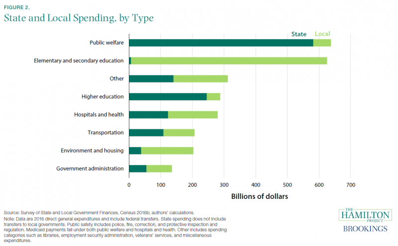
State and local government direct general expenditures are spread across an array of activities, as depicted in figure 2. The largest category is public welfare, which includes spending on means-tested programs such as Temporary Aid for Needy Families, Medicaid, and others, and is predominantly a state-level concern.[6] Only slightly less money is allocated to K–12 education, where during the 2017 school year local governments employed fully 7.5 million people across the country.[7] State governments provided the bulk of funding for higher education, accounting for almost 85 percent of total state and local spending (BLS 2017b).
States have been facing recent budgetary pressures, due in large part to rising Medicaid costs and public employee health and retirement costs (Podkul and Gillers 2018). These expenditures—which fall under public welfare, other, and health and hospitals in figure 2—can crowd out state spending on other important priorities such as higher education (Seltzer 2017).
The activities that states fund are in some ways quite similar across the country; most states allocate roughly one fifth of their expenditures to elementary and secondary education (Census 2016b; authors’ calculations). That said, public services are supplied to varying degrees across states and localities; elementary and secondary education spending per pupil varies from $7,000 in Utah to $22,400 in New York (Census 2016a). States have varying capacities to invest in such services and make different choices about the allocation of their fiscal resources.
Chapter 2. Making Effective State and Local Policies
Fact 3: States differ in their use of cost-benefit analysis.
The wide range of state and local government activities discussed in facts 1 and 2 serves as a reminder of the economic importance of making sound policy at the state and local levels. Cost-benefit analysis—an analytical technique that calculates the net impact of a proposal in monetary terms—is an important contributor to evidence-based policymaking. Nevertheless, the technique is used only sporadically at the state and local levels.
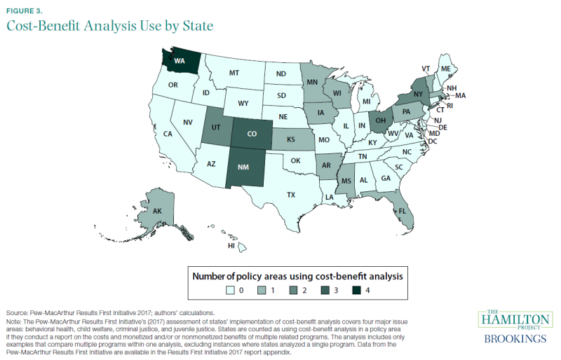
Figure 3 shows the Pew-MacArthur Results First Initiative’s assessment of states’ implementation of cost-benefit analysis across various policy areas: behavioral health, child welfare, criminal justice, and juvenile justice. Notably, Washington, New Mexico, and Colorado are states that use cost-benefit analysis in at least three policy areas, whereas California and Georgia are among the large group of states that do not use it at all.
One example of states implementing cost-benefit analysis is Florida’s Program Accountability Measures initiative, a legislatively required evaluation program, which assesses the costs and benefits of its juvenile justice programs and helps determine which programs are working and warrant additional funding (Pew-MacArthur Results First Initiative 2017). Another example comes from Colorado’s Department of Regulatory Agencies, which is responsible for conducting cost-benefit analyses of existing and proposed regulations (Colorado Department of Regulator Agencies n.d.).[8]
Cost-benefit analysis is applied unevenly across policy areas: from 2008 to 2011, 30 states analyzed questions related to economic development, and 28 states did so for environmental policies, but only 7 conducted housing cost-benefit analyses (Pew-MacArthur Results First Initiative 2013). Reasons for a lack of state and local cost-benefit analysis include staff resource constraints, difficulty integrating it into legislative calendars, and low policymaker demand (Pew-MacArthur Results First Initiative 2013). However, in a Hamilton Project proposal that could help overcome some of these challenges, Justine Hastings (2019) explains how states can use their administrative data to make better policy decisions.
In facts 4 and 5, we present two policy areas that illustrate the need for evidence-based policymaking at the state and local levels.
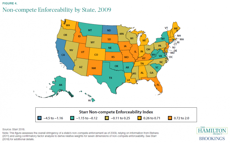
Fact 4: Non-compete enforcement rules are particularly employer friendly in some states.
In the U.S. federal system, many regulatory policies of great economic importance are made at the state (e.g., occupational licensing) and local levels (e.g., land-use rules). These jurisdictions have implicitly made very different assessments of the problems they face, leading to policies that work quite differently across the country.
One important example is the enforcement of non-compete agreements between workers and firms. These agreements prevent employees from taking new jobs at competing employers, thereby limiting workers’ outside employment options and mobility. As shown in figure 4, the vast majority of states enforce these agreements—California being a notable exception—albeit to widely varying degrees. This has resulted in a patchwork of policies across the country: states like Florida (shown in orange) enforce non-competes in a relatively employer-friendly manner, while other states (shown in blue) do not enforce them at all. Some states, like Virginia, enforce non-competes but do so in a way that is relatively worker friendly.
Figure 4 is based on an index created by Evan Starr (2018) that serves as a summary of different dimensions of non-compete enforceability.[9] One important dimension is the willingness of states to allow ex-post modification of non-compete contracts during litigation. Certain states, like Florida and New York, allow the employer-friendly practice of court modification and enforcement of non-compete contracts during litigation if the contract is found to be inconsistent with state law (usually by virtue of being written too broadly). Because the threat of non-compete enforcement—rather than actual litigation—is central to its effects on workers, these policy choices are important (Marx and Nunn 2018; U.S. Department of the Treasury 2016). In other states, like Wisconsin, a contract provision that is inconsistent with state law renders the entire agreement unenforceable.
A second relevant dimension of non-compete enforceability is the requirement that firms provide their existing workers with legal consideration (i.e., a benefit such as a cash bonus, training, a raise, or a promotion) in exchange for agreeing to a non-compete contract. The law in most states is that simply continuing to employ a worker constitutes legal consideration, which is also an employer-friendly practice.
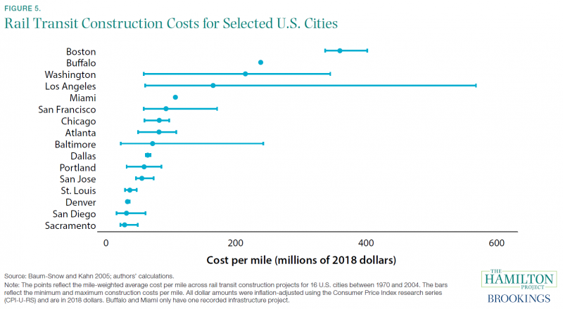
Fact 5: The cost of building new rail infrastructure is both high and variable across the United States.
State and local governments are responsible for more than three-quarters of government spending on infrastructure (Congressional Budget Office 2018), making their activities pivotal for these important investments. Strikingly, the United States incurs substantially higher infrastructure investment costs than other advanced economies (Gordon and Schleicher 2015; Rosenthal 2017). For example, light rail in France has generally cost between $40 million to $100 million per mile, compared with more than $100 million per mile in the United States; underground rail costs in the European Union range from $200–500 million per mile, compared with $2.1 billion per mile for New York City’s Second Avenue subway extension (based on surveys of costs done by Levy 2018).
Figure 5 highlights just how expensive and variable these construction projects can be in the United States, with average costs per mile in Boston more than 12 times the cost per mile in Sacramento. Even within cities, there is wide variation in the cost per mile across projects; in Los Angeles, costs range from $59 million to $566 million per mile. Costs depend importantly on whether the rail system is underground or above ground, but also vary across cities based on contracting and regulatory costs.
Infrastructure projects often stretch across jurisdictions and localities with different regulatory processes, creating an overlapping thicket of regulations through which infrastructure projects must pass. This can present challenges for financing, regulation, and coordination purposes (Gillette 2001), while adding to overall costs (Long 2017). Examples of these problems abound. For water infrastructure repair, regulations sometimes restrict the kinds of materials that can be used, limiting procurement competition and raising costs (Anderson 2018). Partly as a result of state and federal regulations, public buses are more expensive to procure and their fuel economy is unresponsive to price changes (Li, Kahn, and Nickelsburg 2015). And a New York Times report on the Second Avenue Subway (Rosenthal 2017) noted both how work rules raised labor costs and contracting rules pushed costs well above typical rates.
It is important to note that though these regulatory and bureaucratic barriers can add to the costs of infrastructure projects, many still play a crucial role in ensuring that the public is protected from potentially unsafe construction practices or from environmental damages (DeGood 2018). Nevertheless, a more-streamlined process that incorporates some elements of evidence-based policymaking, including cost-benefit analysis, could help lower costs while also protecting workers and the public, especially when different regulations aimed at similar goals may impose overlapping burdens.
Chapter 3. Geographic Access to Employment
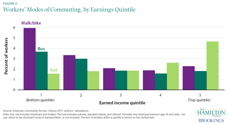
Fact 6: Low-income workers are more likely to use bus transit and less likely to use rail.
Transportation infrastructure is used in different ways by low- and high-income workers, as shown in figure 6. The vast majority of workers—84 percent—commute to work by car. However, given the high cost of buying and owning a car, low-income households need to spend a much higher share of their incomes on vehicles; on average, the top decile spends less than one fifth as much (as a fraction of income) as the bottom decile of households (Bureau of Labor Statistics 2017a; authors’ calculations).
Traditionally, middle- and high-income people have taken advantage of more-expensive, faster transportation technologies to be able to live further from city centers (Glaeser, Kahn, and Rappaport 2008; LeRoy and Sonstelie 1983). When adjusting for other factors, high-income commuters are more likely to drive to work than lower-income workers (Census 2017; authors’ calculations). They are also more likely to use rail (light green bars in figure 6).
Low-income workers are more likely than others to (1) walk or ride a bicycle or (2) ride a bus to work (respectively, the purple and dark green bars in figure 6). Nevertheless, commuting by car is still the dominant mode of commuting, even for workers in the bottom quintile of earnings (77 percent of whom commute by car).
In spite of higher rates of commuting by bus, walking, and biking, which may be slower than taking a train, average commute times are lower for low-income workers (20 minutes) than for high-income ones (29 minutes) (Census 2017; authors’ calculations).[10] However, this does not necessarily indicate that low-income workers have easy access to places with the best job opportunities for them; rather, it could reflect the quality, price, and availability of housing and transportation options, as well as smaller low-skilled labor market returns to traveling long distances. Public policy could assist low-income workers in accessing economic opportunity by improving the functioning of the bus system, as described in a Hamilton Project policy memo by Matthew Turner (2019).
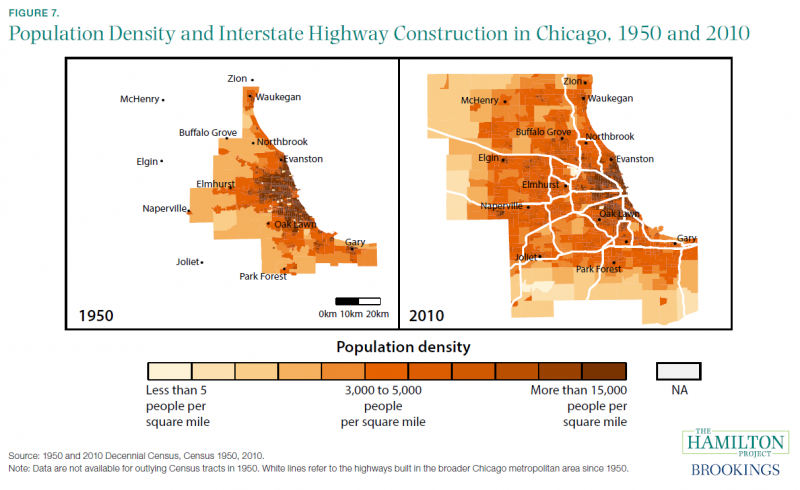
Fact 7: Transportation infrastructure underlies the growth of large metropolitan areas.
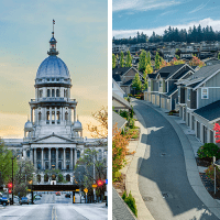
Transportation infrastructure has always been at the center of the evolving economic landscape of the United States. Innovations like canals, railroads, and the Interstate Highway System have continually reduced the costs of moving people and goods between places (Baum-Snow 2007; Donaldson and Hornbeck 2016). Transportation infrastructure underlies the development of large, dense hubs of economic activity like Chicago, whose population density in 1950 and 2010 is shown in the left and right panels, respectively, of figure 7. In 1950, before construction began on the Interstate Highway System, the population of Chicago and the surrounding areas was concentrated closer to the center of the city.[11] (The more densely populated areas outside the central city correspond to rail lines.) However, with the introduction of seven major interstate highways in the subsequent decades, which also correspond to preexisting railroads, the population was able to spread out into the Chicago suburbs and exurbs.
In addition to population, transportation infrastructure shifts economic activity from one place to another; an interstate highway connection placed in a county increases output there but lowers it by a similar amount in adjacent counties (Chandra and Thompson 2000). Highway connections also facilitate enhanced specialization by raising demand for either low- or high-skilled labor, depending on the original skill mix in the county (Michaels 2008).
The construction of the Interstate Highway System, which began in the late 1950s, had profound consequences for the overall distribution of work and population in the United States. By enabling commutes over longer distances, the system caused population dispersal and suburbanization, with each new highway reducing a central city’s population by 18 percent (Baum-Snow 2007) while also causing employment dispersion (Baum-Snow 2010).[12]
In spite of the economic benefits that came with the expansion of the Interstate Highway System, choices about highway routes have also had pernicious effects on low-income and minority communities. For example, the construction of interstate highways in Chicago facilitated white flight and segregation as well as seizures of residential property, resulting in socially and economically isolated communities (Connerly 2002; Hardy, Logan, and Parman 2018; Semuels 2016).
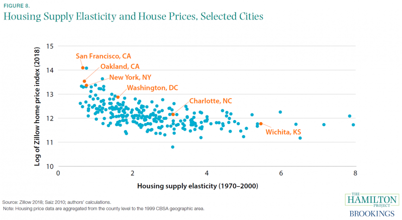
Fact 8: Places where housing is hard to build tend to have higher housing prices.
In most of the United States, housing prices follow the rule of thumb often suggested for homebuyers: homes in the typical neighborhood are valued at less than three times household income (Murray and Schuetz 2018). But in a collection of places—for example, New York City and San Francisco—housing is much more expensive. Land in the centers of these cities is especially expensive; center-city prices are 21 times the prices only 10 miles away. By contrast, for all U.S. cities, center-city prices are only 4 times higher than those on the periphery (Albouy, Ehrlich, and Shin 2018).
Local housing markets vary widely across the country, with large differences in house prices as well as the number of housing units available. Throughout most of the country, housing supply is elastic with respect to changes in price; a small increase in housing prices leads to increases in the housing stock (Saiz 2010). But in many high-priced cities, housing supply is relatively inelastic, meaning that even a large rise in price does not lead to much increase in the housing stock.
Figure 8 depicts this relationship, showing housing prices on the vertical axis and the estimated housing supply elasticity on the horizontal axis. Locations like New York City, Oakland, and San Francisco have both high prices and low housing supply elasticities, indicating that housing supply is slow to adjust and is likely constrained by some combination of physical, economic, and regulatory factors (Paciorek 2013; Saiz 2010). Although some locations have low elasticities and low prices, all the high-priced cities have low elasticities. In these places, increases in demand for housing are not met by sufficient increases in supply, pushing up prices.
Limited housing supply growth, along with increased prices, can make it more difficult for individuals to move to high-productivity areas in search of new and better-paying jobs. Recent research indicates that migration within the United States, and particularly from struggling to prospering areas, has been impeded by housing market constraints, as discussed further in fact 9 (Ganong and Shoag 2017; Nunn, Parsons, and Shambaugh 2018). Geographic mobility throughout the United States has declined over the past 40 years (Molloy et al. 2016).[13] These declines have made the United States a more disconnected economy, and thus it is more difficult to conduct countercyclical monetary and fiscal policy (Schleicher 2017).
Fact 9: Land-use restrictions make housing more expensive.
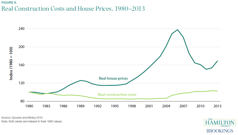
In competitive markets, the prices of used goods are typically constrained by what it costs to produce a new equivalent. In the case of housing, prices could be expected to closely track the cost of acquiring land and constructing a new house. Indeed, for much of the country, housing prices have historically been closely tethered to construction prices (Glaeser and Gyourko 2003). It is therefore striking that the inflation-adjusted price of housing in the United States has risen far faster than construction costs since 1980, as demonstrated by Gyourko and Molloy (2015) and shown in figure 9. Although construction costs have remained roughly stable, the price of land has increased dramatically (Nichols, Oliner, and Mullhall 2013).[14]
The increasing price of land is not entirely due to geographic and space constraints such as steep slopes or coastlines that make it hard to build, although this does play an important role (Saiz 2010). As Gyourko and Molloy (2015) point out, it is generally possible—in a physical sense—to build higher-density housing, allowing for more housing units on a given piece of land. Instead, legal restrictions on the use of land and the construction of new housing have driven increases in housing prices, particularly in places like New York City and San Francisco, and a decrease in housing supply elasticity, as discussed in fact 8 (Glaeser, Gyourko, and Saks 2005, 2006).
When a given place experiences an increase in labor demand, employment rises, fueled in large part by in-migration from the rest of the country. Some places are better able to accommodate labor demand shocks than others. In the long run, the employment response is about 10 percent higher in places with unrestrictive land-use rules than in places with restrictive regulations (Saks 2008). Most research shows that more-stringent residential land-use regulations restrict housing supply elasticity, resulting in higher housing prices and less construction (Gyourko and Molloy 2015). The higher prices in booming cities can make it difficult for new workers to move to these cities, thereby lowering economic growth and opportunity for the country overall. Overly restrictive land-use rules are substantial impediments to accessing high-wage employment, as discussed in a Hamilton Project proposal by Daniel Shoag (2019). These supply constraints develop in part because homeowners have incentives to limit new development that might decrease their home values (Fischel 2001; Gyourko and Molloy 2015).
Endnotes
[1] State and local governments account for a substantially higher share of economic output than does the federal government. Government contributions to 2017 GDP—as opposed to total spending, which includes transfers—were 6.5 percent at the federal level and 10.8 percent at the state and local levels.
[2] Intergovernmental transfers make up about 39 and 33 percent of local and state government revenue, respectively (BEA 2017; authors’ calculations). For local governments, this estimate includes transfers from states.
[3] For more granular analysis of state and local revenues and expenditures and in figure 2, we rely on estimates of direct general expenditures (expenditures that exclude government-run liquor stores, utilities, and social insurance trusts) from the U.S. Census Bureau’s Annual Survey of State and Local Government Finances (Census 2016b).
[4] Although New Hampshire and Oregon collect no sales taxes, they do collect excise taxes.
[5] Direct general expenditures are not directly comparable to the total expenditures figures presented in fact 1 and figure 1, as they come from different surveys. See endnote 3 for more details.
[6] Medicaid, which accounts for nearly 30 percent of state budgets, falls under both public welfare and hospitals and health (MACPAC n.d.).
[7] The 2017 school year is defined as September 2016 through June 2017, and the data are identified using NAICS code 6111 (employment in elementary and secondary schools). The average for these months is 7.5 million. Note that this number includes all staff employed by local governments in elementary and secondary schools; for teachers, specifically, public employment is around 3.2 million (National Center for Education Statistics 2017).
[8] The Colorado Department of Regulatory Agencies has a particularly important role in assessing occupational licensing policies (Kleiner 2015).
[9] This index is based on rules that were in place in 2009. In particular, it does not incorporate subsequent reforms carried out in states like Illinois and Massachusetts that limited the use of non-compete agreements or those in Georgia that made enforcement more employer friendly. See the Hamilton Project proposals by Marx (2018) and Krueger and Posner (2018) for details on these agreements and suggestions for how to reform their use.
[10] This pattern remains even when adjusting for differences between metropolitan areas, and also when restricting survey samples to commuters who travel by car.
[11] Data from the 1950 census are only available for certain counties and census tracts. However, when comparing census tracts that are unavailable in 1950 with those for which data are available in 1960, we still see low population densities in outlying census tracts.
[12] The introduction of subway systems resulted in similar population dispersion (Gonzalez-Navarro and Turner 2018). At the same time, increases in density around defunct streetcar infrastructure have been extremely persistent (Brooks and Lutz 2016).
[13] Mobility has declined in the United States for a variety of reasons, ranging from population aging to declining start-up rates that diminish job-to-job transitions to declining labor market returns to job transitions (Molloy et al. 2016), as well as possible shifts in the jobs available to lower-skilled workers in large, expensive cities (Autor 2019).
[14] However, construction costs do seem to have risen since the mid-2000s (Romem 2018).