
This Hamilton Project policy memo provides ten economic facts highlighting recent trends in crime and incarceration in the United States. Specifically, it explores the characteristics of criminal offenders and victims; the historically unprecedented level of incarceration in the United States; and evidence on both the fiscal and social implications of current policy on taxpayers and those imprisoned.
Read the full introduction
Crime and high rates of incarceration impose tremendous costs on society, with lasting negative effects on individuals, families, and communities. Rates of crime in the United States have been falling steadily, but still constitute a serious economic and social challenge. At the same time, the incarceration rate in the United States is so high—more than 700 out of every 100,000 people are incarcerated—that both crime scholars and policymakers alike question whether, for nonviolent criminals in particular, the social costs of incarceration exceed the social benefits.
While there is significant focus on America's incarceration policies, it is important to consider that crime continues to be a concern for policymakers, particularly at the state and local levels. Public spending on fighting crime—including the costs of incarceration, policing, and judicial and legal services—as well as private spending by households and businesses is substantial. There are also tremendous costs to the victims of crime, such as medical costs, lost earnings, and an overall loss in quality of life. Crime also stymies economic growth. For example, exposure to violence can inhibit effective schooling and other developmental outcomes (Burdick-Will 2013; Sharkey et al. 2012). Crime can induce citizens to migrate; economists estimate that each nonfatal violent crime reduces a city's population by approximately one person, and each homicide reduces a city's population by seventy persons (Cullen and Levitt 1999; Ludwig and Cook 2000). To the extent that migration diminishes a locality's tax and consumer base, departures threaten a city's ability to effectively educate children, provide social services, and maintain a vibrant economy.
The good news is that crime rates in the United States have been falling steadily since the 1990s, reversing an upward trend from the 1960s through the 1980s. There does not appear to be a consensus among scholars about how to account for the overall sharp decline, but contributing factors may include increased policing, rising incarceration rates, and the waning of the crack epidemic that was prevalent in the 1980s and early 1990s.
Despite the ongoing decline in crime, the incarceration rate in the United States remains at a historically unprecedented level. This high incarceration rate can have profound effects on society; research has shown that incarceration may impede employment and marriage prospects among former inmates, increase poverty depth and behavioral problems among their children, and amplify the spread of communicable diseases among disproportionately impacted communities (Raphael 2007). These effects are especially prevalent within disadvantaged communities and among those demographic groups that are more likely to face incarceration, namely young minority males. In addition, this high rate of incarceration is expensive for both federal and state governments. On average, in 2012, it cost more than $29,000 to house an inmate in federal prison (Congressional Research Service 2013). In total, the United States spent over $80 billion on corrections expenditures in 2010, with more than 90 percent of these expenditures occurring at the state and local levels (Kyckelhahn and Martin 2013).
A founding principle of The Hamilton Project's economic strategy is that long-term prosperity is best achieved by fostering economic growth and broad participation in that growth. Elevated rates of crime and incarceration directly work against these principles, marginalizing individuals, devastating affected communities, and perpetuating inequality. In this spirit, we offer “Ten Economic Facts about Crime and Incarceration in the United States” to bring attention to recent trends in crime and incarceration, the characteristics of those who commit crimes and those who are incarcerated, and the social and economic costs of current policy.
- Chapter 1 describes recent crime trends in the United States and the characteristics of criminal offenders and victims.
- Chapter 2 focuses on the growth of mass incarceration in America.
- Chapter 3 presents evidence on the economic and social costs of current crime and incarceration policy.
Chapter 1. The Landscape of Crime in the United States
Crime rates in the United States have been on a steady decline since the 1990s. Despite this improvement, particular demographic groups still exhibit high rates of criminal activity while others remain especially likely to be victims of crime.
Fact 1. Crime rates have steadily declined over the past twenty-five years.
After a significant explosion in crime rates between the 1960s and the 1980s, the United States has experienced a steady decline in crime rates over the past twenty-five years. As illustrated in figure 1, crime rates fell nearly 30 percent between 1991 and 2001, and subsequently fell an additional 22 percent between 2001 and 2012. This measure, calculated by the FBI, incorporates both violent crimes (e.g., murder and aggravated assault) and property crimes (e.g., burglary and larceny-theft). Individually, rates of property and violent crime have followed similar trends, falling 29 percent and 33 percent, respectively, between 1991 and 2001 (U.S. Department of Justice [DOJ] 2010b).
Social scientists have struggled to provide adequate explanations for the sharp and persistent decline in crime rates. Economists have focused on a few potential factors—including an increased number of police on the streets, rising rates of incarceration, and the waning of the crack epidemic—to explain the drop in crime (Levitt 2004). In the 1990s, police officers per capita increased by approximately 14 percent. During this same decade, sentencing policies grew stricter and the U.S. prison population swelled, which had both deterrence (i.e., prevention of further crime by increasing the threat of punishment) and incapacitation (i.e., the inability to commit a crime because of being imprisoned) effects on criminals (Abrams 2011; Johnson and Raphael 2012; Levitt 2004). The waning of the crack epidemic reduced crime primarily through a decline in the homicide rates associated with crack markets in the late 1980s.
Though crime rates have fallen, they remain an important policy issue. In particular, some communities, often those with lowincome residents, still experience elevated rates of certain types of crime despite the national decline.
Figure 1. Crime Rate in the United States, 1960–2012
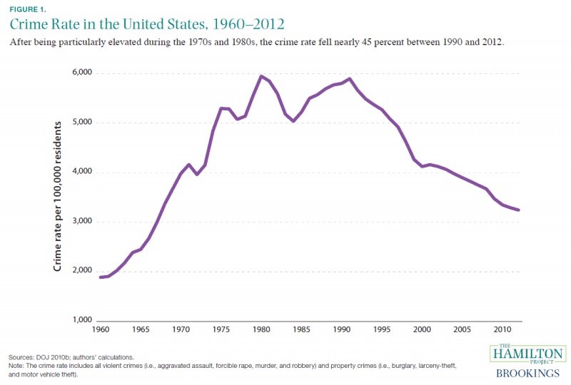
Source: DOJ 2010b; authors' calculations.
Note: The crime rate includes all violent crimes (i.e., aggravated assault, forcible rape, murder, and robbery) and property crimes (i.e., burglary, larceny-theft, and motor vehicle theft).
Fact 2. Low-income individuals are more likely than higher-income individuals to be victims of crime.
Across all types of personal crimes, victimization rates are significantly higher for individuals living in low-income households, as shown in figure 2. In 2008, the latest year for which data are available, the victimization rate for all personal crimes among individuals with family incomes of less than $15,000 was over three times the rate of those with family incomes of $75,000 or more (DOJ 2010a). The most prevalent crime for low-income victims was assault, followed closely by acts of attempted violence, at 33 victims and 28 victims per 1,000 residents, respectively. For those in the higher-income bracket, these rates were significantly lower at only 11 victims and 9 victims per 1,000 residents, respectively.
Because crime tends to concentrate in disadvantaged areas, low-income individuals living in these communities are even more likely to be victims. Notably, evidence from the Moving to Opportunity program—a multiyear federal research demonstration project that combined rental assistance with housing counseling to help families with very low incomes move from areas with a high concentration of poverty—suggests that moving into a less-poor neighborhood significantly reduces child criminal victimization rates. In particular, children of families that moved as a result of receiving both a housing voucher to move to a new location and counseling assistance experienced personal crime victimization rates that were 13 percentage points lower than those who did not receive any voucher or assistance (Katz, Kling, and Liebman 2000).
Victims of personal crimes face both tangible costs, including medical costs, lost earnings, and costs related to victim assistance programs, and intangible costs, such as pain, suffering, and lost quality of life (Miller, Cohen, and Wiersama 1996). There are also public health consequences to crime victimization. Since homicide rates are so high for young African American men, men in this demographic group lose more years of life before age sixtyfive to homicide than they do to heart disease, which is the nation's overall leading killer (Heller et al. 2013).
Figure 2. Victimization Rates for Persons Age 12 or Older, by Type of Crime and Annual Family Income, 2008
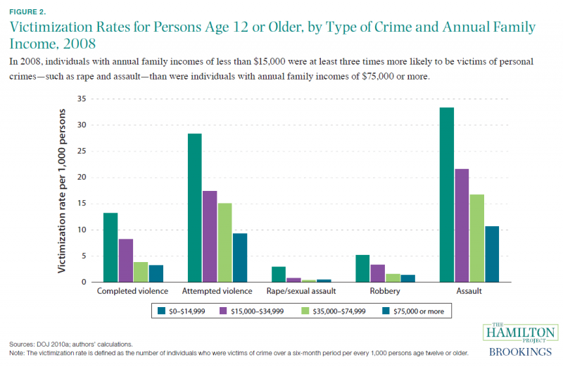
Source: DOJ 2010a; authors' calculations.
Note: The victimization rate is defined as the number of individuals who were victims of crime over a six-month period for every 100,000 U.S. residents.
Fact 3. The majority of criminal offenders are younger than age thirty.
Juveniles make up a significant portion of offenders each year. More than one quarter (27 percent) of known offenders—defined as individuals with at least one identifiable characteristic that were involved in a crime incident, whether or not an arrest was made—were individuals ages eleven to twenty, and an additional 34 percent were ages twenty-one to thirty; all other individuals composed fewer than 40 percent of offenders. As seen in figure 3, this trend holds for all types of crimes. More specifically, 55 percent of offenders committing crimes against persons (such as assault and sex offenses) were ages eleven to thirty. For crimes against property (such as larceny-theft and vandalism) and crimes against society (including drug offenses and weapon law violations), 63 percent and 66 percent of offenders, respectively, were individuals in the eleven-to-thirty age group.
A stark difference in the number of offenders by gender is also evident. Most crimes—whether against persons, property, or society—are committed by men; of criminal offenders with known gender, 72 percent are male. This trend for gender follows for crimes against persons (73 percent), crimes against property (70 percent), and crimes against society (77 percent) (DOJ 2012). Combined, these facts indicate that most offenders in the United States are young men.
Some social scientists explain this age profile of crime by appealing to a biological perspective on criminal behavior, focusing on the impaired decision-making capabilities of the adolescent brain in particular. There are also numerous social theories that emphasize youth susceptibility to societal pressures, namely their concern with identity formation, peer reactions, and establishing their independence (O'Donoghue and Rabin 2001).
Figure 3. Number of Offenders in the United States, by Age and Offense Category, 2012
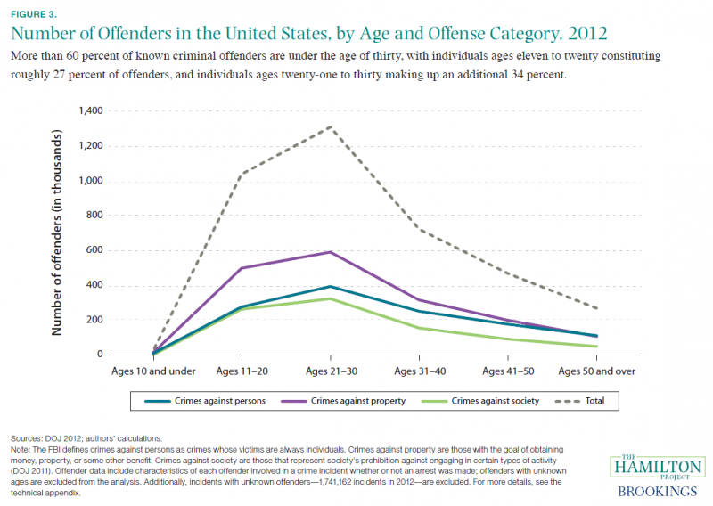
Source: DOJ 2012; authors' calculations.
Note: The FBI defines crimes against persons as crimes whose victims are always individuals. Crimes against property are those with the goal of obtaining money, property, or some other benefit. Crimes against society are those that represent society's prohibition against engaging in certain types of activity, and are typically victimless crimes (DOJ 2011). Offender data include characteristics of each offender involved in a crime incident whether or not an arrest has been made; offenders with unknown ages are excluded from the analysis. Additionally, incidents with unknown offenders—1,741,162 incidents in 2012—are excluded. For more details, see the technical appendix.
Fact 4. Disadvantaged youths engage in riskier criminal behavior.
Youths from low-income families (those with incomes at or below 200 percent of the federal poverty level) are equally likely to commit drug-related offenses than are their higher-income counterparts. As seen in figure 4, low-income youths are just as likely to use marijuana by age sixteen, and to use other drugs or sell drugs by age eighteen. In contrast, low-income youths are more likely to engage in violent and property crimes than are youths from middle- and highincome families. In particular, low-income youths are significantly more likely to attack someone or get into a fight, join a gang, or steal something worth more than $50. In other words, youths from lowincome families are more likely to engage in crimes that involve or affect other people than are youths from higher-income families.
A standard economics explanation for the socioeconomic profile of property crime is that for poor youths the attractiveness of alternatives to crime is low: if employment opportunities are limited for teens living in poor neighborhoods, then property crime becomes relatively more attractive. The heightened likelihood of violent crime among poor youths raises the issue of automatic behaviors—in other words, youths intuitively responding to perceived threats—which has become the focus of recent research in this field. However, the similar rates of drug use across teens from different income groups is consistent with a more general model of risky teenage activity associated with the so-called impaired decision-making capabilities of the adolescent brain.
Some intriguing recent academic work has proposed that adverse youth outcomes are often the result of quick errors in judgment and decision-making. In particular, hostile attribution bias—hypervigilance to threat cues and the tendency to overattribute malevolent intent to others—appears to be more common among disadvantaged youths, partly because these youths grow up with a heightened risk of having experienced abuse (Dodge, Bates, and Pettit 1990; Heller et al. 2013). Some experts have consequently begun promoting cognitive behavioral therapy for these youths to help them recognize and rewire the automatic behaviors and biased beliefs that often result in judgment and decision-making errors. Promising results from several experiments in Chicago—in particular, improved schooling outcomes and fewer arrests for violent crimes—suggest that it is possible to change the outcomes of disadvantaged youths simply by helping them recognize when their automatic responses may trigger negative outcomes (Heller et al. 2013).
Figure 4. Adolescent Risk Behaviors by Family Income Level
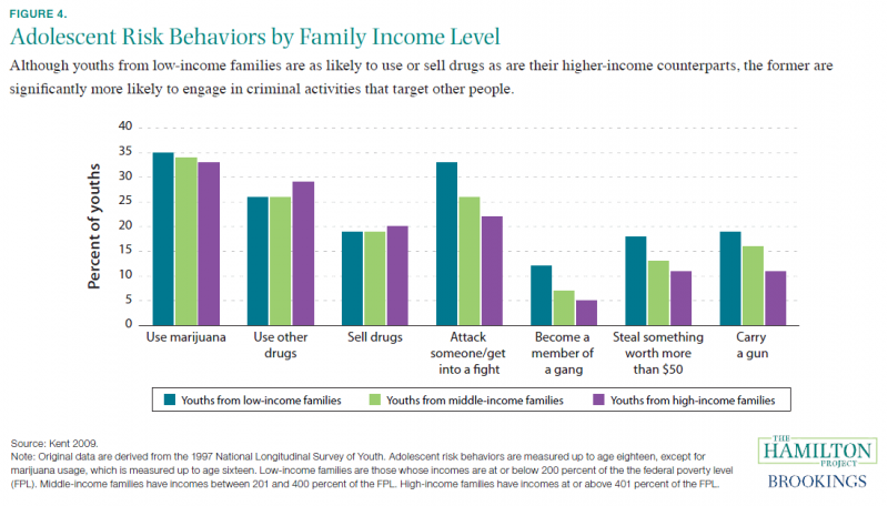
Source: Kent 2009.
Note: Original data are derived from the 1997 National Longitudinal Survey of Youth. Adolescent risk behaviors are measured up to age eighteen, except for marijuana usage, which is measured up to age sixteen. Low-income families are those whose incomes are at or below 200 percent of the FPL. Middle-income families have incomes between 201 and 400 percent of the FPL. High-income families have incomes at or above 401 percent of the FPL.
Chapter 2. The Growth of Mass Incarceration in America
The incarceration rate in the United States is now at a historically unprecedented level and is far above the typical rate in other developed countries. As a result, imprisonment has become an inevitable reality for subsets of the American population.
Fact 5. Federal and state policies have driven up the incarceration rate over the past thirty years.
The incarceration rate in the United States—defined as the number of inmates in local jails, state prisons, federal prisons, and privately operated facilities per every 100,000 U.S. residents—increased during the past three decades, from 220 in 1980 to 756 in 2008, before retreating slightly to 710 in 2012 (as seen in figure 5).
The incarceration rate is driven by three factors: crime rates, the number of prison sentences per number of crimes committed, and expected time served in prison among those sentenced (Raphael 2011). Academic evidence suggests that increases in crime cannot explain the growth in the incarceration rate since the 1980s (Raphael and Stoll 2013). However, the likelihood that an arrested offender will be sent to prison, as well as the time prisoners can expect to serve, has increased for all types of crime (Raphael and Stoll 2009, 2013). Given that both the likelihood of going to prison and sentence lengths are heavily influenced by adjudication outcomes and the types of punishment levied, most of the growth in the incarceration rate can be attributed to changes in policy (Raphael and Stoll 2013).
Policymakers at the federal and state levels have created a stricter criminal justice system in the past three decades. For example, state laws and federal laws—such as the Sentencing Reform Act of 1984—established greater structure in sentencing through specified guidelines for each offense. Additionally, between 1975 and 2002,all fifty states adopted some form of mandatory-sentencing law specifying minimum prison sentences for specific offenses. In fact, nearly three quarters of states and the federal government—through laws like the Anti-Drug Abuse Act of 1986—enacted mandatory sentencing laws for possession or trafficking of illegal drugs. Many states also adopted repeat offender laws, known as “three strikes” laws, which strengthened the sentences of those with prior felony convictions. These policies, among others, are believed to have made the United States tougher on those who commit crime, raising the incarceration rate through increased admissions and longer sentences (Raphael and Stoll 2013).
The continued growth in the federal prison population stands in contrast to recent trends in state prison populations. Between 2008 and 2012, the number of inmates in state correctional facilities decreased by approximately 4 percent (from roughly 1.41 million to 1.35 million), while the number of inmates in federal prisons increased by more than 8 percent (from approximately 201,000 to nearly 218,000) (Carson and Golinelli 2013). This increase in federal imprisonment rates has been driven by increases in immigrationrelated admissions. Between 2003 and 2011, admissions to federal prisons for immigration-related offenses increased by 83 percent, rising from 13,100 to 23,939 (DOJ n.d.).
Figure 5. Incarceration Rate in the United States, 1960–2012
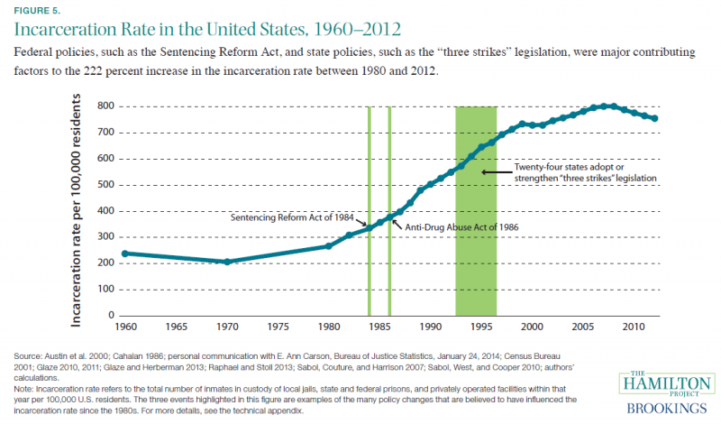
Source: Austin et al. 2000; Cahalan 1986; Carson forthcoming; Census Bureau 2001; Glaze 2010, 2011; Glaze and Herberman 2013; Raphael and Stoll 2013; Sabol, Couture, and Harrison 2007; Sabol, West, and Cooper 2010; authors' calculations.
Note: Incarceration rate refers to the total number of inmates in custody of local jails, state or federal prisons, or privately operated facilities within the year per 100,000 U.S. residents. The three events highlighted in this figure are examples of the many policy changes that are believed to have influenced incarceration rates since the 1980s. For more details, see the technical appendix.
Fact 6. The U.S. incarceration rate is more than six times that of the typical OECD nation.
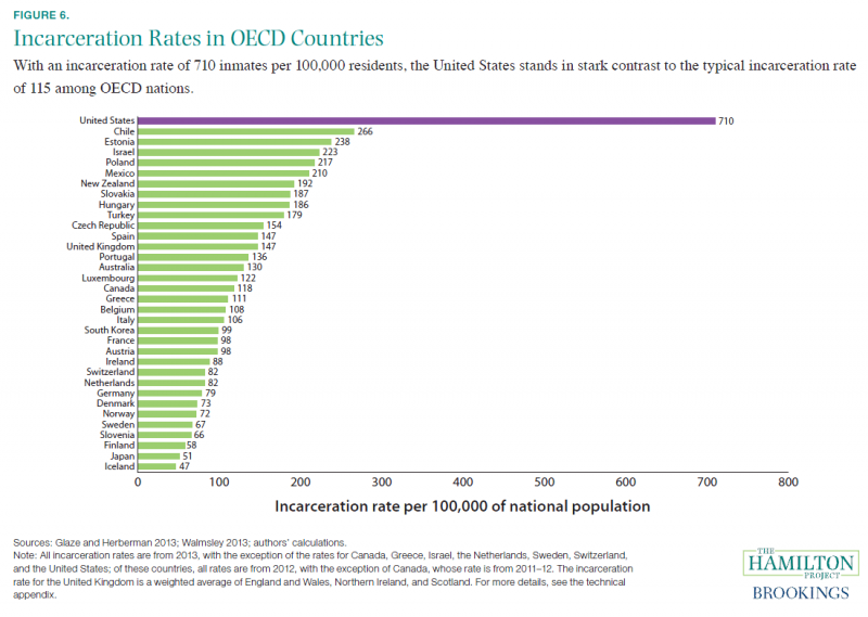
The United States is an international outlier when it comes to incarceration rates. In 2012, the incarceration rate in the United States—which includes inmates in the custody of local jails, state or federal prisons, and privately operated facilities—was 710 per 100,000 U.S. residents (Glaze and Herberman 2013). This puts the U.S. incarceration rate at more than five times the typical global rate of 130, and more than twice the incarceration rate of 90 percent of the world's countries (Walmsley 2013).
The U.S. incarceration rate in 2012 was significantly higher than those of its neighbors: Canada's and Mexico's incarceration rates were 118 and 210, respectively. Moreover, the U.S. incarceration rate is more than six times higher than the typical rate of 115 for a nation in the Organisation for Economic Co-Operation and Development (OECD) (Walmsley 2013). As seen in figure 6, in recent years incarceration rates in OECD nations have ranged from 47 to 266; these rates are relatively comparable to the rates seen in the United States prior to the 1980s. Indeed, mass incarceration appears to be a relatively unique and recent American phenomenon.
A variety of factors can explain the discrepancy in incarceration rates. One important factor is higher crime rates, especially rates of violent crimes: the homicide rate in the United States is approximately four times the typical rate among the nations in figure 6 (United Nations Office on Drugs and Crime 2014). Additionally, drug control policies in the United States—which have largely not been replicated in other Western countries—have prominently contributed to the rising incarcerated population over the past several decades (Donahue, Ewing, and Peloquin 2011). Another important factor is sentencing policy; in particular, the United States imposes much longer prison sentences for drug-related offenses than do many economically similar nations. For example, the average expected time served for drug offenses is twenty-three months in the United States, in contrast to twelve months in England and Wales and seven months in France (Lynch and Pridemore 2011).
Figure 6. Incarceration Rates in OECD Countries
Fact 7. There is nearly a 70 percent chance that an African American man without a high school diploma will be imprisoned by his mid-thirties.
For certain demographic groups, incarceration has become a fact of life. Figure 7 illustrates the cumulative risk of imprisonment for men by race, education, and birth cohort. As described by Pettit and Western (2004), the cumulative risk of imprisonment is the projected lifetime likelihood of serving time for a person born in a specific year. Specifically, each point reflects the percent chance that a man born within a given range of years will have spent time in prison by age thirty to thirty-four. Notably, most men who are ever incarcerated enter prison for the first time before age thirty-five, and so these cumulative risks by age thirty to thirty-four are reflective of lifetime risks.
Men in the first birth cohort, 1945–49, reached their mid-thirties by 1980 just as the incarceration rate began a steady incline. For all education levels within this age group, only an 8-percentage point differential separated white and African American men in terms of imprisonment risk (depicted by the difference between the two solid lines on the far left of figure 7). As the incarceration rate rose, however,discrepancies between races became more apparent. Men born in the latest birth cohort, 1975–79, reached their mid-thirties around 2010; for this cohort, the difference in cumulative risk of imprisonment between white and African American men is more than double the difference for the first birth cohort (as seen on the far right of figure 7).
These racial disparities become particularly striking when considering men with low educational attainment. Over 53 percentage points distance white and African American male high school dropouts in the latest birth cohort (depicted by the difference between the two dashed lines on the far right of figure 7), with male African American high school dropouts facing a nearly 70 percent cumulative risk of imprisonment. This high risk of imprisonment translates into a higher chance of being in prison than of being employed. For African American men in general, it translates into a higher chance of spending time in prison than of graduating with a four-year college degree (Pettit 2012; Pettit and Western 2004).
Figure 7. Cumulative Risk of Imprisonment by Age 30–34 for Men Born Between 1945–49 and 1975–79, by Race and Education
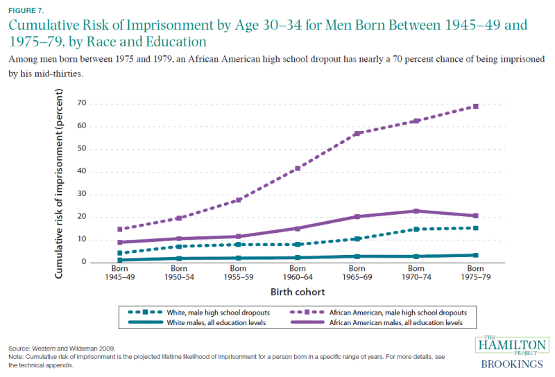
Source: Western and Wildeman 2009.
Note: Cumulative risk of imprisonment is the projected lifetime likelihood of imprisonment for a person born in a specific range of years. For more details, see the technical appendix.
Chapter 3. The Economic and Social Costs of Crime and Incarceration
Today's high rate of incarceration is considerably costly to American taxpayers, with state governments bearing the bulk of the fiscal burden. In addition to these budgetary costs, current incarceration policy generates economic and social costs for both those imprisoned and their families.
Fact 8. Per capita expenditures on corrections more than tripled over the past thirty years.
In 2010, the United States spent more than $80 billion on corrections expenditures at the federal, state, and local levels. Corrections expenditures fund the supervision, confinement, and rehabilitation of adults and juveniles convicted of offenses against the law, and the confinement of persons awaiting trial and adjudication (Kyckelhahn 2013). As figure 8 illustrates, total corrections expenditures more than quadrupled over the past twenty years in real terms, from approximately $17 billion in 1980 to more than $80 billion in 2010. When including expenditures for police protection and judicial and legal services, the direct costs of crime rise to $261 billion (Kyckelhahn and Martin 2013).
Most corrections expenditures have historically occurred at the state level and continue to do so. As shown in figure 8, in 2010, more than 57 percent of direct cash outlays for corrections came from state governments, compared to 10 percent from the federal government and nearly 33 percent from local governments. Increased expenditures at every level of government are not surprising given the growth in incarceration, which has far outstripped population growth, leading to a higher rate of incarceration and higher corrections spending per capita (Census Bureau 2001, 2013; Raphael and Stoll 2013). Per capita expenditures on corrections (denoted by the dashed line in figure 8) more than tripled between 1980 and 2010. In real terms, each U.S. resident on average contributed $260 to corrections expenditures in 2010, which stands in stark contrast to the $77 each resident contributed in 1980.
Crime-related expenditures generate a significant strain on state and federal budgets, leading some to question whether public funds are best spent incarcerating nonviolent criminals. Preliminary evidence from the recent policy experience in California—in which a substantial number of nonviolent criminals were released from state and federal prisons—suggests that alternatives to incarceration for nonviolent offenders (e.g., electronic monitoring and house arrest) can lead to slightly higher rates of property crime, but have no statistically significant impact on violent crime (Lofstrom and Raphael 2013). These conclusions have led some experts to suggest that public safety priorities could better be achieved by incarcerating fewer nonviolent criminals, combined with spending more on education and policing (ibid.).
Figure 8. Total Corrections Expenditures by Level of Government and Per Capita Expenditures, 1980–2010
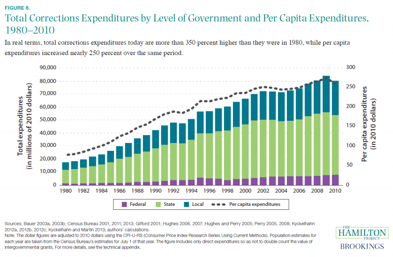
Source: Bauer 2003a, 2003b; Census Bureau 2001, 2011, 2013; Gifford 2001; Hughes 2006, 2007; Hughes and Perry 2005; Perry 2005, 2008; Kyckelhahn 2012a, 2012b, 2012c; Kyckelhahn and Martin 2013; authors' calculations.
Note: The dollar figures were adjusted to 2010 dollars using the CPI-U-RS (Consumer Price Index Research Series Using Current Methods). Population estimates for each year are taken from the Census Bureau's estimates for July 1 of that year. The figure includes only direct expenditures so as not to double count the value of intergovernmental grants. For more details, see the technical appendix.
Fact 9. By their fourteenth birthday, African American children whose fathers do not have a high school diploma are more likely than not to see their fathers incarcerated.
In 2010, approximately 2.7 million children, or over 3 percent of all children in the United States, had a parent in prison (The Pew Charitable Trusts 2010). As of 2007, an estimated 53 percent of prisoners in the United States were parents of children under age eighteen, a majority being fathers (Glaze and Maruschak 2010). Furthermore, it is not the case that these parents were already disengaged from their children's lives. For example, in 2007, approximately half of parents in state prisons were the primary provider of financial support for their children—and nearly half had lived with their children—prior to incarceration (ibid.). Furthermore, fathers often are required to pay child support during their incarceration, and since they make little to no money during their incarceration, they often accumulate child support debt.
Figure 9 illustrates the cumulative risk of imprisonment for parents—or the projected lifetime likelihood of serving time for a person born in a specific year—by the time their child turns fourteen, by child's race and their own educational attainment (Wildeman 2009). Regardless of race, fathers are much more likely to be imprisoned than are mothers. These risks of imprisonment are magnified when parental educational attainment is taken into account; high school dropouts are much more likely to be imprisoned than are individuals with higher levels of education. Fathers who are high school dropouts face a cumulative risk of imprisonment that is approximately four times higher than that of fathers with some college education. An African American child with a father who dropped out of high school has more than a 50 percent chance of seeing that father incarcerated by the time the child reaches age fourteen.
Young children (ages two to six) and school-aged children of incarcerated parents have been shown to have emotional problems and to demonstrate weak academic performance and behavioral problems, respectively. It is unclear, however, the extent to which these problems result from having an incarcerated parent as opposed to stemming from the other risk factors faced by families of incarcerated individuals; incarcerated parents tend to have low levels of education and high rates of poverty, in addition to frequently having issues with drugs, alcohol, and mental illness (Center for Research on Child Wellbeing 2008).
Figure 9. Cumulative Risk of Parent's Imprisonment for Children by Age 14, by Race and Parent's Education
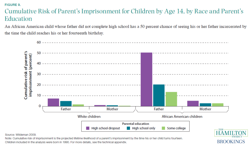
Source: Wildeman 2009.
Note: Cumulative risk of imprisonment is the projected lifetime likelihood of a parent's imprisonment by the time his or her child turns fourteen. Children included in the analysis were born in 1990. For more details, see the technical appendix.
Fact 10. Juvenile incarceration can have lasting impacts on a young person's future.
After increasing steadily between 1975 and 1999, the rate of youth confinement began declining in 2000, with the decline accelerating in recent years (Annie E. Casey Foundation 2013). In 2011, there were 64,423 detained youths, a rate of roughly 2 out of every 1,000 juveniles ages ten and older (Sickmund et al. 2013). Detained juveniles include those placed in a facility as part of a court-ordered disposition (68 percent); juveniles awaiting a court hearing, adjudication, disposition, or placement elsewhere (31 percent); and juveniles who were voluntarily admitted to a facility in lieu of adjudication as part of a diversion agreement (1 percent) (ibid.).
Youths are incarcerated for a variety of crimes. In 2011, 22,964 juveniles (37 percent of juvenile detainees) were detained for a violent offense, and 14,705 (24 percent) were detained for a property offense. More than 70 percent of youth offenders are detained in public facilities, for which the cost is estimated to be approximately $240 per person each day, or around $88,000 per person each year (Petteruti, Walsh, and Velazquez 2009).
In addition to these direct costs, juvenile detention is believed to have significant effects on a youth's future since it jeopardizes his or her accumulation of human and social capital during an important developmental stage. Studies have found it difficult to estimate this effect, given that incarcerated juveniles differ across many dimensions from those who are not incarcerated. Aizer and Doyle (2013) overcome this difficulty by using randomly assigned judges to estimate the difference in adult outcomes between youths sent to juvenile detention and youths who were charged with a similar crime, but who were not sent to juvenile detention. The authors find that sending a youth to juvenile detention has a significant negative impact on that youth's adult outcomes. As illustrated in figure 10, juvenile incarceration is estimated to decrease the likelihood of high school graduation by 13 percentage points and increase the likelihood of incarceration as an adult by 22 percentage points. In particular, those who are incarcerated as juveniles are 15 percentage points more likely to be incarcerated as adults for violent crimes or 14 percentage points more likely to be incarcerated as adults for property crimes.
Figure 10. Effect of Juvenile Incarceration on Likelihood of High School Graduation and Adult Imprisonment
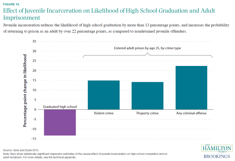
Source: Aizer and Doyle 2013.
Note: Bars show statistically significant regression estimates of the causal effect of juvenile incarceration on high school completion and on adult recidivism. For more details, see the technical appendix.