Introduction
Between December 2007 and June 2009 the United States experienced the most severe recession in the postwar period. The over 4 percent decline in gross domestic product (GDP) was only reversed more than three years after the beginning of the recession. During the worst part of the Great Recession, virtually every segment of the U.S. economy was adversely affected. Employment losses were severe, but also unevenly distributed: men, the young, and the less educated suffered disproportionately in the recession’s aftermath.
Read Full Introduction
Before the Great Recession, macroeconomists had chronicled a Great Moderation—a reduction in the volatility of the business cycle—achieved by the judicious use of monetary policy (Clarida, Galí, and Gertler 2000; Galí and Gambetti 2009). Now, in the wake of the most severe downturn and the slowest recovery in the postwar period, it seems that such talk was premature.
Given the massive human cost of recessions, it is incumbent upon policy makers to assess the policy tools at their disposal and identify those that are most effective at hastening economic recovery during a downturn. In this document we describe how different groups of workers were affected by the Great Recession, what works in fiscal stimulus, what could be done differently in future recessions, and the fiscal preparedness of states for the next downturn.
There are two sets of policy tools used to foster recovery following recessions: monetary policy and fiscal policy. Monetary policy, consisting of actions taken by the Federal Reserve, is used to keep interest rates low and reduce unemployment during and after a recession. Fiscal policy includes various forms of government spending and tax cuts enacted by Congress. Following a recession, both sets of policy tools can be used to increase demand, thereby raising output and more quickly returning the economy to prerecession conditions.
To be most effective, it is crucial that stimulus be expeditious. In the Great Recession, a portion of the fiscal policy response occurred automatically within preexisting programs. These programs are called “automatic stabilizers” because they provide immediate stimulus during a recession without requiring action from Congress. For this reason, automatic stabilizers like unemployment insurance (UI), the Supplemental Nutrition Assistance Program (SNAP, formerly Food Stamps), and Medicaid—in addition to automatic stabilization associated with tax revenue—are particularly valuable.
As soon as a recession arrives, participation in these programs expands as incomes fall and unemployment rises—and in some cases, participation increases because of automatically reduced eligibility requirements for participants. The result is that additional funds are automatically disbursed (or taxes reduced), immediately providing fiscal stimulus. The United States makes considerable use of automatic stabilizers, which amounted to about 2 percentage points of GDP during the depths of the Great Recession (Congressional Budget Office [CBO] 2016a).
Monetary policy makers were also quick to react. As the Great Recession began and GDP and employment plunged, the Federal Reserve reduced the federal funds rate. (The federal funds rate is the interest rate that banks charge each other on a particular kind of overnight loan.) This conventional monetary policy action aimed to lower borrowing costs for individuals and businesses, thereby encouraging both immediate consumption and investment. However, the ongoing very low federal funds rate—which cannot be lowered much farther—and the severity of the Great Recession prompted an increased focus on fiscal policy as a recession-fighting tool.
Fiscal stimulus that requires congressional action takes longer. In some cases it may take a considerable amount of time to observe that a recession has begun, debate the appropriate legislative response, pass legislation, disburse funds to states and individuals, and finally spend authorized funds. Such lags are perhaps inevitable, but quick delivery of stimulus is preferable for both the economy and the affected workers and families. The American Recovery and Reinvestment Act of 2009 (ARRA) was a major vehicle for such fiscal stimulus, authorizing spending on infrastructure, health care, and education; expanding automatic stabilizers; and making various tax cuts.
With unemployment and poverty spiking, two major programs—UI and Temporary Assistance for Needy Families (TANF)—responded in starkly different ways. UI claims shot up in response to the increasing number of the newly unemployed, buffering eligible workers against earnings losses. Not all of the newly unemployed were eligible for UI, but the program was broadly successful in achieving its mission. By contrast, the caseload of TANF—the successor to Aid to Families with Dependent Children—barely increased as poverty grew. Though TANF plays a role in alleviating deep poverty, it is not currently structured to respond effectively to cyclical poverty variation or to act as an automatic stabilizer.
The fiscal stimulus in ARRA is widely believed to have reduced the severity of the Great Recession (Chodorow-Reich et al. 2012; CBO 2015). By the CBO’s estimate, the fiscal stimulus bill caused GDP to be 0.4 to 2.3 percent higher in 2011 than it otherwise would have been (CBO 2015). But which components of the fiscal stimulus were most useful? Stimulus aimed at low-income or otherwise cash-constrained households tends to be more effective, whereas business tax cuts tend to be less effective (Whalen and Reichling 2015). By some calculations, government spending is typically a more effective stimulus than tax cuts, partially because workers tend to spend only a fraction of stimulus provided through the tax system. Across all stimulus types, it is widely believed that fiscal stimulus is more effective during recessions and less effective during expansions (Auerbach and Gorodnichenko 2012; Fazzari, Morley, and Panovska 2014), likely because downturns are characterized by slack in both labor and capital markets (i.e., available resources are not fully employed), allowing fiscal stimulus to increase total output.
Despite all of the monetary and fiscal actions taken to mitigate the severity of the Great Recession, output has still not returned to either its prerecession trend or to potential output (CBO 2016b). Unemployment has only recently recovered to a level close to the prerecession rate, and other measures of labor market slack, such as the fraction of workers who work part time for economic reasons, remain elevated (Bureau of Labor Statistics [BLS] 2016a). In addition, states are not adequately prepared for the next recession. In most states, rainy-day funds remain insufficient to cope with a large, unexpected decline in tax revenues. These states will either need to cut crucial government services—hurting both state residents and the broader economy—or rely on the federal government for support to maintain their budgets.
A founding principle of The Hamilton Project’s economic strategy is that long-term prosperity is best achieved by fostering economic growth and broad participation in that growth. To that end, The Hamilton Project offers the following nine facts about the Great Recession and the kinds of fiscal stimulus that can help mitigate the severity of future recessions.
Fact 1: The Great Recession was unprecedented in the postwar period for its severity and duration.
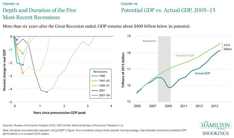
Between December 2007 and June 2009, the United States experienced the most severe recession in the postwar period. Recessions are conventionally measured by declines in GDP, which measures overall economic activity and is defined as the value of the economy’s total output of goods and services. Figure 1a compares the depth and duration of the Great Recession with the four most recent recessions, plotting the changes in GDP from the first quarter of the recession to the quarter when GDP was the lowest relative to the beginning of the recession (bold lines) and the economy’s subsequent recoveries (light lines). Not only was the Great Recession (grey) deeper than any recent recession, but it look nearly four years for the economy to regain the prerecession GDP level—twice as long as for the 1981–82 recession. As discussed in The Hamilton Project jobs gap analysis, the labor market was slower to recover following the Great Recession than it was after previous downturns (Kearney and Hershbein 2015), and still remains weaker in May 2016 than it was before the recession (The Hamilton Project n.d.). This continues a pattern in which successive recessions have been followed by more-prolonged job-market recoveries—reflecting long-term structural changes in the economy as well as cyclical factors (Kearney and Hershbein 2015).
During the Great Recession, the nation’s actual GDP contracted by more than 4 percent. How much of a reduction was this relative to the economy’s hypothetical capacity, or “potential GDP”? Potential GDP refers to the economy’s maximum sustainable output, which mirrors GDP under normal conditions and to which actual GDP is expected to return quickly after a downturn. Today—more than six years after the recession ended—economic output remains substantially below potential GDP. As shown in figure 1b, the gap between actual and potential GDP reached its widest point in the third quarter of 2009, when the economy fell short of potential GDP by $1.2 trillion in constant 2015 dollars, or 7 percent of potential GDP. The financial stabilization and fiscal stimulus policies enacted during the recession helped mitigate the severity of the downturn (Blinder and Zandi 2015), but the gap between actual and potential GDP, at $410 billion in constant 2015 dollars, still had not closed by the fourth quarter of 2015.
Fact 2: Employment losses in the Great Recession were greater among men and the young.
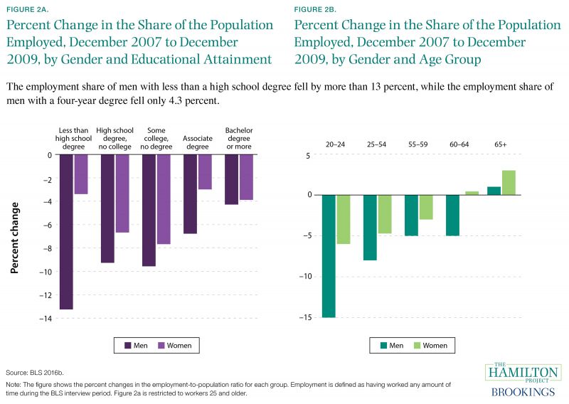
The Great Recession sharply reduced employment for many workers in the United States, but these reductions were concentrated among men, younger workers, and workers with lower levels of education. This may be the result of a so-called job ladder that renders low-skilled workers—and young workers—disproportionately sensitive to the business cycle (Barnichon and Zylberberg 2014; Beaudry, Green, and Sand 2013). Figure 2a shows the change in the employed share of the population aged 25 and older by education level and gender, from just before the recession began (December 2007) to December 2009—roughly the trough of the labor market. Employment fell more sharply for workers with low levels of education, though women with less than a high school degree saw only a 3.4 percent loss in employment. Men tended to experience steeper declines than women, within both education and age groups. The employment share fell the farthest for men without a high school degree; note that men tend to suffer more during recessions largely because they tend to be employed in industries that are more cyclical (Hoynes, Miller, and Schaller 2012).
Figure 2b shows the change in the share of the population employed for different age groups, from December 2007 to December 2009. The steep decline captured by the leftmost bars in figure 2b (corresponding to ages 20–24) highlights the impact of the recession on young people. This pattern partly reflects the option that young people possess to acquire education rather than participate in a weak labor market—an alternative less readily available to middle-aged workers. This pattern may also be attributable to the tendency of firms to lay off inexperienced workers before those in mid-career.
Fact 3: Fiscal stimulus tempered the length and the depth of the Great Recession.
Policy makers rely on two sets of tools to foster recovery following a recession. Monetary policy, consisting of actions taken by the Federal Reserve, is used to keep interest rates low and reduce unemployment during and after a recession. Fiscal policy includes various forms of government spending and tax cuts enacted by Congress. Following a recession, both sets of policies can be used to increase demand, thereby raising output and more quickly returning the economy to prerecession conditions.
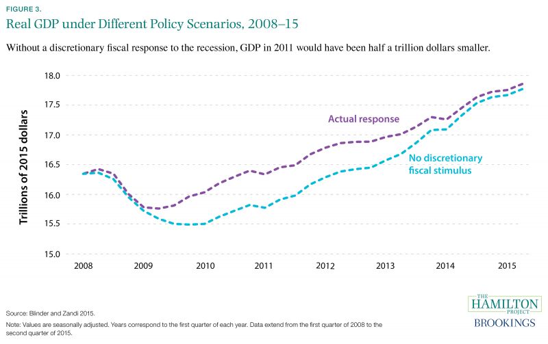
During the Great Recession, fiscal policy played an important role in the economic recovery (figure 3). The purple line shows the actual path of GDP: note that the economy reached its low point in the second quarter of 2009 and then began growing again. Blinder and Zandi (2015) estimate that, absent the fiscal stimulus, the economy would have continued to contract until the fourth quarter of 2009, to $15.5 trillion in output annually (in constant 2015 dollars), and would not have reached prerecession levels until the second quarter of 2012—a year after it actually did.
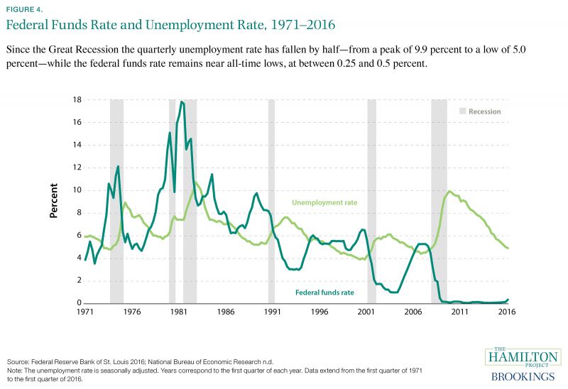
Fact 4: The federal funds rate is near historical lows and cannot be reduced much farther.
As the central banking institution of the United States, the Federal Reserve has two primary responsibilities, often referred to as its dual mandate: (1) to maintain price stability and (2) to help the economy remain near maximum sustainable employment. As shown in figure 4, the unemployment rate rises as the economy contracts: in the past 45 years, as the economy has gone through each recession, unemployment has increased on average by 2.5 percentage points. The Federal Reserve responds to these changes in the labor market by using open-market operations, which consist of the acquisition and sale of securities, to lower the federal funds rate (the interest rate at which institutions lend deposits at the Federal Reserve to other institutions overnight) and recently to expand its balance sheet. When economic conditions worsen, a reduction in the federal funds rate lowers interest rates throughout the economy, encouraging businesses to invest and employ more workers and encouraging consumers to spend more, consequently lowering the unemployment rate.
As shown in figure 4, after the Federal Reserve lowers the federal funds rate, the unemployment rate tends to drop, albeit with a lag. When economic conditions improve, the Federal Reserve raises the federal funds rate again to forestall inflation, which occurs when the economy overheats and prices rise too rapidly.
The unemployment rate remained elevated well after the end of the Great Recession, and the Federal Reserve has consequently kept the federal funds rate close to zero for some time, while also pursuing other expansionary monetary policies to encourage economic activity. If another recession were to occur while the federal funds rate remains near zero, the Federal Reserve would not have its conventional arsenal of tools since the federal funds rate cannot be lowered much farther. It would then have to make do with unconventional tools to help the economy recover. Given that considerable uncertainty remains about the effectiveness and costs of unconventional monetary policies, expansionary fiscal policy may be an attractive option.
Fact 5: Many spending programs provided highly effective stimulus during the Great Recession.
Governments may use fiscal policy—additional government spending or tax cuts—to stimulate the economy during a recession. A fiscal multiplier is an estimate of the increased output caused by a given increase in government pending or reduction in taxes. Any multiplier greater than zero implies that additional government spending (or reduced taxes) adds to total output. Fiscal multipliers greater than one indicate an increase in private-sector output along with an increase in output from government spending.
Although there is disagreement among economists over the exact size of various fiscal multipliers (see Auerbach, Gale, and Harris [2010] for a discussion), multipliers are generally believed to be higher during recessions than they are under normal economic conditions when the economy is near its full potential (Auerbach and Gorodnichenko 2012; Fazzari, Morley, and Panovska 2014; see Ramey and Zubairy 2014 for a dissenting view). This is likely because downturns are characterized by slack in both labor and capital markets (i.e., available resources are not fully employed), thereby allowing fiscal stimulus to increase total output. Multipliers are also higher when the spending program or tax cut targets lower-income people, who are more likely to spend the stimulus (Parker et al. 2013; Whalen and Reichling 2015).
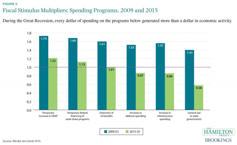
Not all spending or tax cuts are created equal, as indicated by the variation in fiscal multipliers shown in figure 5 and figure 6. But during the depths of the recession, each spending multiplier analyzed by Blinder and Zandi (2015) was greater than one, indicating that spending on these programs raised output by more than their costs. Moreover, during the recent recession, every spending multiplier featured here was higher than the tax multipliers described in Fact 6. Note that the multipliers reported here are broadly similar to those estimated by CBO (Whalen and Reichling 2015).
As shown in figure 5, the most stimulative type of spending during the recession was a temporary increase in the SNAP maximum benefit: for every $1 increase in government spending, total output increased by $1.74. Work-share programs and UI benefit extensions were also relatively stimulative. Consistent with economic theory, the programs with the largest multipliers were those directed at low-income or newly unemployed people. More recently, as the economy has improved, the multipliers have diminished. However, the multipliers for SNAP benefits, workshare programs, and UI benefits remain above one, indicating that these programs remain effective as forms of stimulus, generating additional private-sector economic activity.
Fact 6: Well-targeted tax cuts can stimulate the economy.
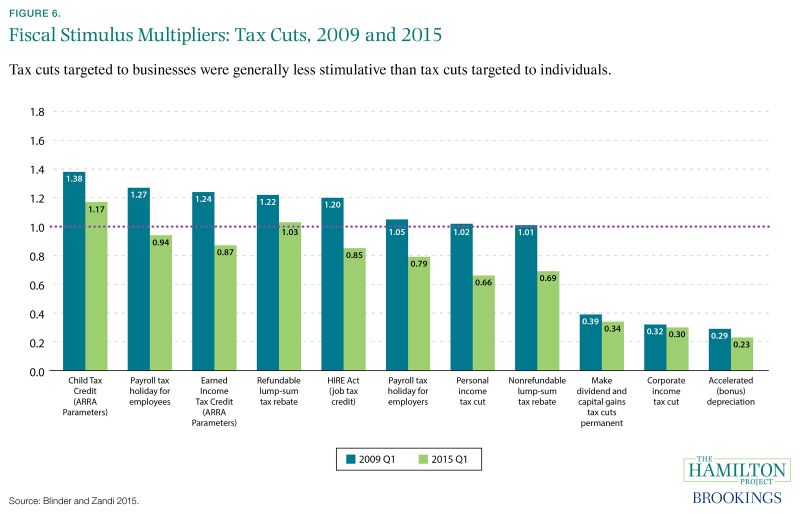
Tax cuts can also provide useful stimulus, though multiplier estimates are generally lower and more variable than estimates for spending programs. Estimates range from 1.38 for the Child Tax Credit in the midst of the recession to 0.23 in 2015 for accelerated depreciation, which effectively allows firms to postpone tax liabilities.
Although many tax cuts had a fiscal multiplier greater than one during the recession, in 2015 only the multipliers for the Child Tax Credit and refundable lump sum tax rebate were still greater than one. Furthermore, their values were smaller than those for spending multipliers (Fact 5) such as increasing SNAP benefits and extending UI benefits. Spending programs or tax cuts that focus on lower-income people tend to have higher multipliers because those people are more likely than higher-income people to spend what they receive. In addition, policies such as accelerated depreciation and cuts in the corporate tax rate, both of which benefit businesses, are less stimulative than tax cuts for individuals.
Fact 7: Automatic stabilizers generate substantial, well-timed stimulus.
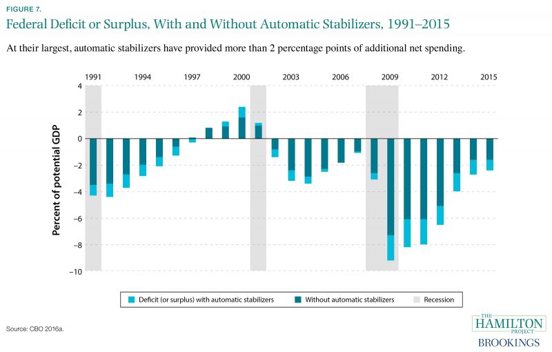
Fiscal stimulus may take two forms during a recession. The first is discretionary, when Congress authorizes new tax cuts or government spending to shore up the economy (as it did with the passage of the ARRA in 2009). However, some fiscal stimulus also occurs automatically without congressional action, making for a quicker response to deteriorating economic conditions. For example, as employment and income levels decline during economic downturns, participation in existing safety net programs increases and affected households’ tax bills fall. According to the CBO, three types of outlays constitute the large majority of automatic stabilization in federal spending: UI benefits, Medicaid benefits, and SNAP benefits (Russek and Kowalewski 2015). In addition, there are several sources of revenue that contribute to automatic stabilization: individual income taxes, taxes on corporate profits, Social Security and Medicare payroll taxes, taxes on production and imports, and UI taxes. During expansions, rising incomes generate more tax revenue; during downturns, taxes are automatically lowered as incomes fall. These automatic stabilizers help to moderate the booms and busts of the business cycle, increasing aggregate demand to offset the negative effects of an economic downturn, and decreasing demand once the economy has recovered.
As shown in figure 7, spending on automatic stabilizers varies over the business cycle, expanding promptly during recessions. This stands in contrast to discretionary fiscal policy: by the time that ARRA was authorized in 2009—five quarters after the start of the recession—spending on automatic stabilizers had already grown by 2 percent of GDP.
Fact 8: Safety net programs varied widely in their effectiveness as automatic stabilizers during the Great Recession.
Poverty and economic hardship typically increase in recessions and decrease in economic expansions. In particular, households with few resources are especially affected by the business cycle. Among poor households, the effect of the Great Recession was particularly severe relative to previous recessions. Bitler and Hoynes (2015) estimate that for a 1 percentage point increase in the unemployment rate, the share of households below 50 percent of the poverty threshold expanded more in the Great Recession than during the two recessions of the early 1980s. (The poverty threshold in 2015 was $24,036 for a family of four with two children [U.S. Census Bureau 2016b].) The safety net plays an important role in mitigating these effects, partly by automatically expanding during economic downturns as eligibility for safety net programs increases. However, there were stark differences among safety net programs in their responsiveness to the Great Recession.
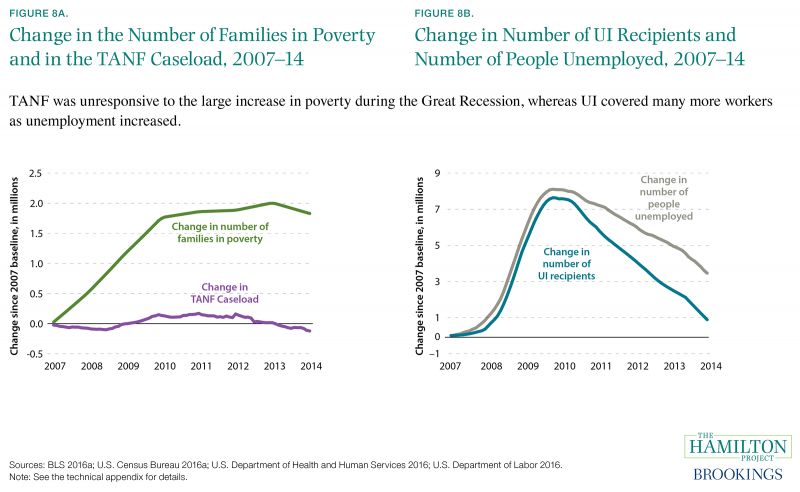
For example, the TANF program—which supports poor families with cash assistance, resources for child care, and work-related services, among others—expanded only slightly during the most-recent recession, and the number of families benefiting from the program has now fallen below its prerecession level, despite the fact that poverty remains elevated. Figure 8a shows the cumulative change in the TANF caseload (purple line) during and after the recession compared with the cumulative change in the number of families in poverty (green line); the dramatic split between the two lines suggests that TANF is failing to reach many needy families. Unlike SNAP and UI, TANF is largely funded through a federal block grant with a fixed value, making it less responsive to changes in need.
Other programs, including SNAP and UI, functioned more effectively as automatic stabilizers during the most-recent recession (Bitler and Hoynes 2010; Di Maggio and Kermani 2016). Note that during the Great Recession, Congress increased spending on SNAP and UI above and beyond the increase that would have occurred automatically. Figure 8b shows the change in the number of UI recipients compared with the change in the number of people unemployed. In contrast to TANF, UI did respond to the economic downturn, although many workers are either ineligible for or do not claim UI, and the program consequently covers only a portion of newly unemployed workers. Despite these limitations, UI was a powerful automatic stabilizer, with the increase in UI recipients amounting to more than 7 million during the economic downturn.
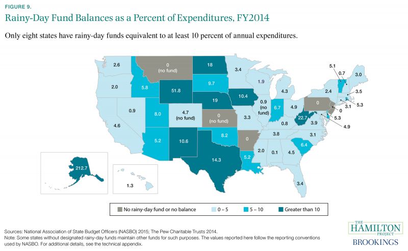
Fact 9: Insufficiently financed rainy-day funds have left the majority of states unprepared for the next recession.
Rainy-day funds—also called budget stabilization funds—are dedicated pools of money set aside by states during good times to help them weather economic downturns. Since states are generally restricted by law from running budget deficits, rainy-day funds help them to balance their budgets when tax revenues fall, without resorting to devastating spending cuts or tax increases at exactly the wrong moment. In each of the previous two recessions, states used their rainy-day funds to avoid more than $20 billion in tax increases and/or cuts to services (McNichol 2014).
Nonetheless, many states still struggle to allocate sufficient savings to rainy-day funds. This can be attributed in part to poor design: 43 states set arbitrary caps or targets on annual contributions to rainy-day funds (The Pew Charitable Trusts 2015), and in many states these caps and targets on contributions are too small. In 2015, six years after the end of the Great Recession, only eight states had accumulated enough in their rainy-day funds to offset a hypothetical one-year loss of 10 percent or more of their annual expenditures. Given that average state taxes dropped 11 percent from fiscal year 2008 to fiscal year 2009, and 21 states experienced losses above 10 percent (The Nelson A. Rockefeller Institute of Government n.d.), many states could struggle to absorb a similar loss in the next recession using rainy-day funds alone.